Functional Maps

Serie of personal notes on functional maps

Info! Unfinished notes

List of related ressources:

• SIGGRAPH 2017 course
• AIM@shape (3D models repository)

Spectral decomposition

``Can you hear the shape of a drum?’’ M. Kac, 1966. No … but …

Eigenfunction decomposition

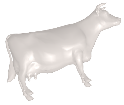
Let us first consider the following shape which is defined as a triangular mesh with $m$ vertices.

The eigenfunctions of the Laplace-Beltrami operator are obtained by solving:

$$\Delta_s \phi_i = \lambda_i \phi_i,$$

where $\Delta_s$ is the Laplace-Beltrami operator¹, $\phi_i$ is the $i^{th}$ eigenfunction and $\lambda_i$ its associated eigenvalues. In practice, we deal with discrete formulations and the $\Delta_s$ is a square matrix noted $L$ (of size $m \times m$ for the source) and the eigenfunctions are represented as eigenvectors $\Phi$ (e.g., a vector of length $m$). This gives us the following formulation: \begin{equation} L \Phi_i = \lambda_i \Phi_i, \label{eq:eigenfunction_decomposition} \end{equation}

Equation \eqref{eq:eigenfunction_decomposition} is then typically solved on a sparse matrix eigensolver and the eigenvectors are then sorted based on the order of the eigenvalues.

What do these eigenfunctions means?

It is possible to visualize the eigenfunctions projected onto the geometries:

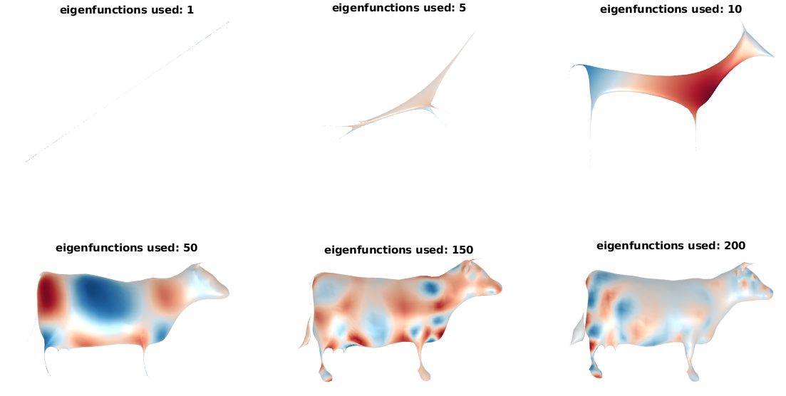
As shown on the figure, after being sorted according to the eigenvalues, the eigenfunctions of the LB operators are ordered from low to high frequencies. This property can be used to apply a low pass filter on the shape. For exemple, we can reconstruct a shape with different number of eigenfunctions²: First, we project the geometry onto each eigenfunction such as:

$$\alpha^x_i \leftarrow \sum_{j=1}^m x_j \Phi_i(j),~~~~~~ \alpha^y_i \leftarrow \sum_{j=1}^m y_j \Phi_i(j),~~~\text{and}~~~ \alpha^z_i \leftarrow \sum_{j=1}^m z_j \Phi_i(j)$$

And the surface reconstruction for $k$ eigenvalues is obtained by:

$$x_j \leftarrow \sum_{i=1}^{k} \alpha_i^x \Phi_i(j),~~~~~~ y_j \leftarrow \sum_{i=1}^{k} \alpha_i^y \Phi_i(j),~~~\text{and}~~~ z_j \leftarrow \sum_{i=1}^{k} \alpha_i^z \Phi_i(j)$$

The final reconstruction with different number of eigenfunction:

Can we do more?

Now given a second shape with $n$ vertices, and its own decomposition formulated similarly such as:

$$\beta^x_i \leftarrow \sum_{j=1}^n x_j' \Phi_i'(j),~~~~~~\beta^y_i \leftarrow \sum_{j=1}^n y_j' \Phi_i'(j),~~~\text{and}~~~\beta^z_i \leftarrow \sum_{j=1}^n z_j' \Phi_i'(j)$$

Levy² mention pose transfert as a potential application ``provided that the $\alpha$’s and the $\beta$’s are expressed in the same langage’’. In this context, the definition of the reconstruction is defined as:

$$x_j \leftarrow \sum_{i=1}^{l} \alpha_i^x \Phi_i'(j) + \sum_{i=l+1}^{k} \beta_i^x \Phi_i'(j)\\ y_j \leftarrow \sum_{i=1}^{l} \alpha_i^y \Phi_i'(j) + \sum_{i=l+1}^{k} \beta_i^y \Phi_i'(j)\\ z_j \leftarrow \sum_{i=1}^{l} \alpha_i^z \Phi_i'(j) + \sum_{i=l+1}^{k} \beta_i^z \Phi_i'(j)$$

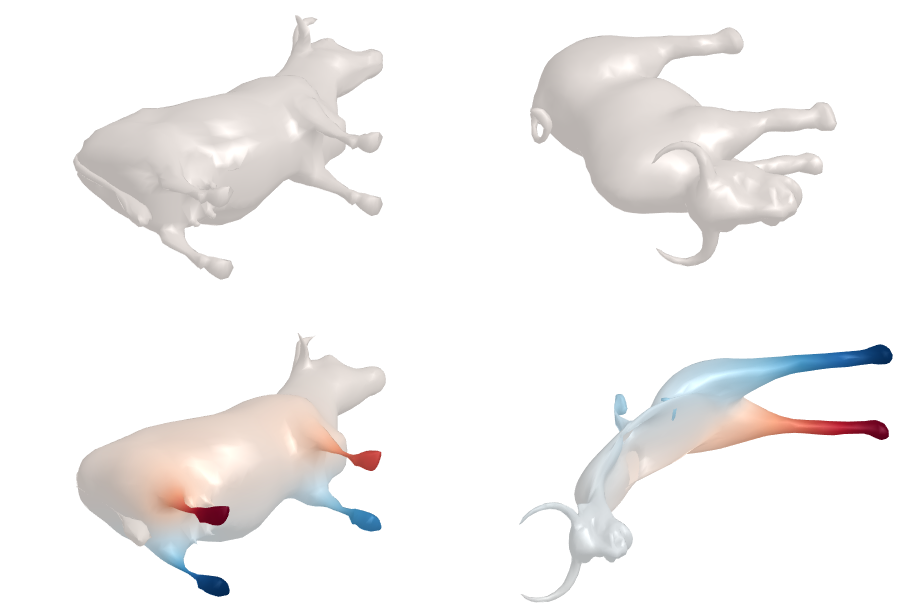
Let’s give it a try by using the 5 first coefficients ($l = 5$) from the cow and apply to a bull:

Why did it fail?

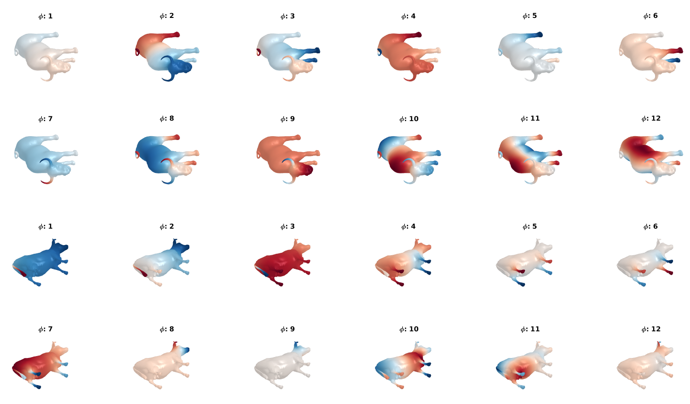
As Levy says in his paper the $\alpha$’s and the $\beta$’s have to be expressed in the same language. Let’s look at the first eigenfunctions to see how they are distributed:

As shown on the figure, some of the eigenfunctions seems to have a good correspondence and some of them are mixted, in other worlds they do not speak the same language. More specifically I hand picked some of the eigenfunctions that have interesing properties in the following figure:

Both $2^{nd}$, $4^{th}$, $5^{th}$, and $10^{th}$ eigenfunctions are a good match. The eigenfunctions 4 (on the bull) and 3 (on the cow) have a good correspondence but are not ordered similarly. Eigenfunctions 8 (on the bull) and 7 (on the cow) are the opposite of each other; this is a well known phenomenon as the eigenfunction decomposition is prone to sign flipping.

As a conclusion, we can consider that the pose transfert did not work because the eigenfunctions do not speak the same language.

Functional maps

Preliminaries and notations

Let consider the matching between two shapes: the source $M$ and the target $N$.

Both the source and the target are defined as a triangular meshes with $m$ and $n$ vertices respectively.

Feature descriptors

Wave Kernel Signature

Heat Kernel Signature

SHOT

See ³

Functional map computation

Features matching

The feature matching is obtained by finding the map which maximize the similarity between the descriptors projected on the eigenfunctions. In other words, we seek to minimize: \begin{equation} C = \arg\min_C \vert\vert CA-B \vert\vert^2 \end{equation}

Regularization terms

The map will be isometric if and only if: \begin{equation} C \Delta_M = \Delta_N C \end{equation}

The mapping will be locally volume preserving if and only if the map is orthonormal which is defined as: \begin{equation} C^T C = Id \end{equation}

The mapping is conformal if and only if: \begin{equation} C^T \Delta_1 C= \Delta_2 \end{equation}

Final cost function

The final functional map that include the feature matching and the regularization term is defined as: \begin{equation} C_{opt} = \arg\min_C \vert\vert CA-B \vert\vert^2 + \vert\vert C \Delta_M - \Delta_N C \vert\vert^2 \end{equation}

References

1. M. Meyer, M. Desbrun, P. Schroder, and A. H. Barr, Discrete Differential-Geometry Operators for Triangulated 2-Manifolds, Springer, 2003. ↩

2. B Levy, Laplace-Beltrami Eigenfunctions Towards an Algorithm That “Understands” Geometry, SMI, 2006 ↩ ↩²

3. , F. Tombari, S. Salti, and L. D. Stefano Unique Signatures of Histograms for Local Surface Description, ECCV, 2010. ↩